17 KiB
JianhuanZhuo
Building a Real-Time Recommendation Engine with Data Science
Editor’s Note: This presentation was given by Nicole White at GraphConnect Europe in April 2016. Here’s a quick review of what she covered:
- Basic graph-powered recommendations
- Social recommendations
- Similarity recommendations
- Cluster recommendations
What we’re going to be talking about today is data science and graph recommendations:
I’ve been with Neo4j for two years now, but have been working with Neo4j and Cypher for three. I discovered this particular graph database when I was a grad student at the University of Texas Austin studying for a masters in statistics with a focus on social networks.
Real-time recommendation engines are one of the most common use cases for Neo4j, and one of the things that makes it so powerful and easy to use. To explore this, I’ll explain how to incorporate statistical methods into these recommendations by using example datasets.
The first will be simple – entirely in Cypher with a focus on social recommendations. Next we’ll look at the similarity recommendation, which involves similarity metrics that can be calculated, and finally a clustering recommendation.
Basic Graph-Powered Recommendations
The following dataset includes food and drink places in the Dallas Fort Worth International Airport, one of the major airport hubs in the United States:
We have place nodes in yellow and are modeling their location in terms of gate and terminal. And we are also categorizing the place in terms of major categories for food and drink. Some include Mexican food, sandwiches, bars and barbecue.
Let’s do a simple recommendation. We want to find a specific type of food in a certain location in the airport, and the curled brackets represent user inputs which are being entered into our hypothetical app:
This English sentence maps really well as a Cypher query:
This is going to pull all the places in the category, terminal and gate the user has requested. Then we get the absolute distance of the place to gate where the user is, and return the results in ascending order. Again, a very simple Cypher recommendation to a user based just on their location in the airport.
Social Recommendations
Let’s look at a social recommendation. In our hypothetical app, we have users who can log in and “like” places in a way similar to Facebook and can also check into places:
Consider this data model on top of the first model that we explored, and now let’s find food and drink places in the following categories closest to some gate in whatever terminal that user’s friends like:
The MATCH clause is very similar to the MATCH clause of our first Cypher query, except now we are matching on likes and friends:
The first three lines are the same, but for the user in question – the user that’s “logged in” – we want to find their friends through the :FRIENDS_WITH relationship along with the places those friends liked. With just a few added lines of Cypher, we are now taking a social aspect into account for our recommendation engine.
Again, we’re only showing categories that the user explicitly asked for that are in the same terminals the user is in. And, of course, we want to filter this by the user who is logged in and making this request, and it returns the name of the place along with its location and category. We are also accounting for how many friends have liked that place and the absolute value of the distance of the place from the gate, all returned in the RETURN clause.
Similarity Recommendation
Now let’s take a look at a similarity recommendation engine:
Similarly to our earlier data model, we have users who can like places, but this time they can also rate places with an integer between one and 10. This is easily modeled in Neo4j by adding a property to the relationship.
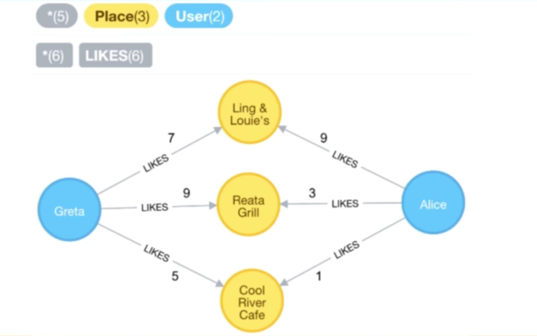
This allows us to find other similar users, like in the example of Greta and Alice. We’ve queried the places they’ve mutually liked, and for each of those places, we can see the weights they have assigned. Presumably, we can use these numbers to determine how similar they are to each other:
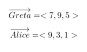
Now we have two vectors:
And now let’s apply Euclidean distance to find the distance between those two vectors:
And when we plug in all the numbers, we get the following similarity metric, which is really the distance metric between the two users:
You can do this between two specific users easily in Cypher, especially if they’ve only mutually liked a small subset of places. Again, here we’re matching on two users, Alice and Greta, and are trying to find places they’ve mutually liked:
They both have to have a :LIKES relationship to the place for it to be found in this result, and then we can easily calculate the Euclidean distance between them with the square root of the sum of their squared differences in Cypher.
While this may work in an example with two specific people, it doesn’t necessarily work in real time when you’re trying to infer similar users from another user on the fly, by comparing them against every other user in the database in real time. Needless to say, this doesn’t work very well.
To find a way around this, we pre-compute this calculation and store it in an actual relationship:
While in large datasets we would do this in batches, in this small example dataset, we can match on a Cartesian product of all the users and places they’ve mutually liked. When we use WHERE id(u1) < id(u2) as part of our Cypher query, this is just a trick to ensure we’re not finding the same pair twice on both the left and the right.
Then with their Euclidean distance and themselves, we’re going to create a relationship between them called :DISTANCE and set a Euclidean property called euclidean. In theory, we could also store other similarity metrics on some relationship between users to capture different similarity metrics, since some might be more useful than others in certain contexts.
And it’s really this ability to model properties on relationships in Neo4j that makes things like this incredibly easy. However, in practice you don’t want to store every single relationship that can possibly exist because you’ll only want to return the top few people of their neighbors.
So you can just store the top in according to some threshold so you don’t have this fully connected graph. This allows you to perform graph database queries like the below in real time, because we’ve pre-computed it and stored it on the relationship, and in Cypher we’ll be able to grab that very quickly:
In this query, we’re matching on places and categories:
Again, the first three lines are the same, except that for the logged-in user, we’re getting users who have a :DISTANCE relationship to them. This is where what we went over earlier comes into play – in practice you should only store the top :DISTANCE relationships to users who are similar to them so you’re not grabbing a huge volume of users in this MATCH clause. Instead, we’re grabbing users who have a :DISTANCE relationship to them where those users like that place.
This has allowed us to express a somewhat complicated pattern in just a few lines. We’re also grabbing the :LIKES relationship and putting it on a variable because we’re going to use those weights later to apply a rating.
What’s important here is that we’re ordering those users by their distance ascending, because it is a distance metric, and we want the lowest distances because that indicates they are the most similar.
With those other users ordered by the Euclidean distance, we’re going to collect the top three users’ ratings and use those as our average score to recommend these places. In other words, we’ve taken an active user, found users who are most similar to them based on the places they’ve liked, and then averaged the scores those similar users have given to rank those places in a result set.
We’re essentially taking an average here by adding it up and dividing by the number of elements in the collection, and we’re ordering by that average ascending. Then secondarily, we’re ordering by the gate distance. Hypothetically, there could be ties I suppose, and then you order by the gate distance and then returning the name, category, gate and terminal.
Cluster Recommendations
Our final example is going to be a cluster recommendation, which can be thought of as a workflow of offline computing that may be required as a workaround in Cypher. This may now be obsolete based on the new procedures announced at GraphConnect Europe, but sometimes you have to do certain algorithmic approaches that Cypher version 2.3 doesn’t expose.
This is where you can use some form of statistical software, pull data out of Neo4j into a software such as Apache Spark, R or Python. Below is an example of R code for pulling data out of Neo4j, running an algorithm, and then – if appropriate – writing the results of that algorithm back into Neo4j as either a property, node, relationship or a new label.
By persisting the results of that algorithm into the graph, you can use it in real-time with queries similar to the ones we just went over:
Below is some example code for how you do this in R, but you can easily do the same thing with whatever software you’re most comfortable with, such as Python or Spark. All you have to do is log in and connect to the graph.
In the following example, I’ve clustered users together based on their similarities. Each user is represented as an observation, and I want to get the average rating that they’ve given each category:
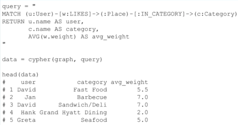
Presumably, users who rate the bar category in similar ways are similar in general. Here I’m grabbing the names of users who like places in the same category, the category name, and the average weight of the “likes” relationships, as average weight, and that’s going to give me a table like this:
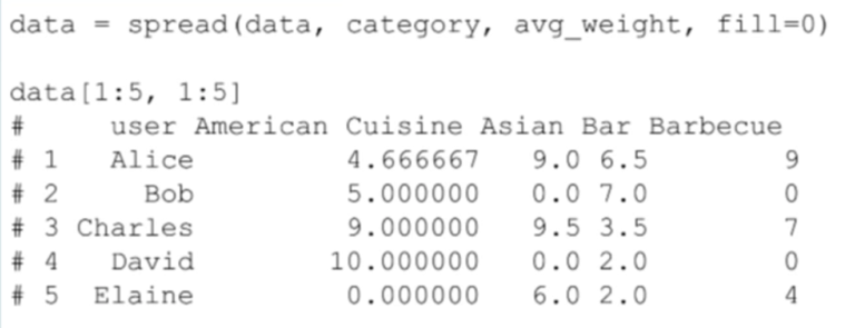
Because we want each user to be an observation, we will have to manipulate the data where each feature is the average weight rating they’ve given restaurants within that category, per category. We’ll then use this to determine how similar they are, and I’m going to use a clustering algorithm to determine users being in different clusters.
In R this is very straightforward:
For this demonstration we are using k-means, which allows you to easily grab cluster assignments. In summary, I ran a clustering algorithm and now for each user I have a cluster assignment.
Bob and David are in the same cluster – they’re in cluster two – and now I’ll be able to see in real time which users have been determined to be in the same cluster.
Next we write it into a CSV, which we then load into the graph:
We have users and cluster assignments, so the CSV will only have two columns. LOAD CSV is a syntax that’s built into Cypher that allows you to call a CSV from some file path or URL and alias it as something. Then we’ll match on the users that already exist in the graph, grab the user column out of that CSV, and merge on the cluster.
Here we’re creating a new labeled node in the graph, the Cluster ID, which was given by k-means. Next we create relationships between the user and the cluster, which allows us to easily query when we get to the actual recommendation users who are in the same cluster.
Now we have a new label cluster where users who are in the same cluster have a relationship to that cluster. Below is what our new data model looks like, which is on top of the other data models we explored:
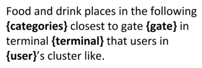
Now let’s consider the following query:
With this Cypher query, we’re going beyond similar users to users in the same cluster. At this point we’ve also deleted those distance relationships:
In this query, we’ve taken the user who’s logged in, finding their cluster based on the user-cluster relationship, and finding their neighbors who are in that same cluster.
We’ve assigned that to some variable cl, and we’re getting other users – which I’ve aliased as a neighbor variable – who have a user-cluster relationship to that same cluster, and then we’re getting the places that neighbor has liked. Again, we’re putting the “likes” on a variable, r, because we’re going want to grab weights off of the relationship to order our results.
All we’ve changed in the query is that instead of using the similarity distance, we’re grabbing users in the same cluster, asserting categories, asserting the terminal and asserting that we’re only grabbing the user who is logged in. We’re collecting all those weights of the :LIKES relationships from their neighbors liking places, getting the category, the absolute value of the distance, ordering that in descending order, and returning those results.
In these examples we’ve been able to take a pretty involved process and persist it in the graph, and then used the results of that algorithm – the results of the clustering algorithm and the clustering assignments – in real time.
Our preferred workflow is to update these clustering assignments however frequently you see fit — for example, nightly or hourly. And, of course, you can use intuition to figure out how often is acceptable to be updating these cluster assignments.
作者:Nicole White 译者:译者ID 校对:校对者ID


