19 KiB
Translating by Chao-zhi 8 best languages to blog about
TL;DR: In this post we’re going to do some metablogging and analyze different blogs popularity against their ranking in Google. All the code is on GitHub repo.
The idea
I’ve been wondering, how many page views actually do different blogs get daily, as well as what programming languages are most popular today among blog reading audience. It was also interesting to me, whether Google ranking of websites directly correlates with their popularity.
In order to answer these questions, I decided to make a Scrapy project that will scrape some data and then perform certain Data Analysis and Data Visualization on the obtained information.
Part I: Scraping
We will use Scrapy for our endeavors, as it provides clean and robust framework for scraping and managing feeds of processed requests. We’ll also use Splash in order to parse Javascript pages we’ll have to deal with. Splash uses its own Web server that acts like a proxy and processes the Javascript response before redirecting it further to our Spider process.
I don’t describe Scrapy project setup here as well as Splash integration. You can find example of Scrapy project backbone here and Scrapy+Splash guide here.
Getting relevant blogs
The first step is obviously getting the data. We’ll need Google search results about programming blogs. See, if we just start scraping Google itself with, let’s say query “Python”, we’ll get lots of other stuff besides blogs. What we need is some kind of filtering that leaves exclusively blogs in the results set. Luckily, there is a thing called Google Custom Search Engine, that achieves exactly that. There’s also this website www.blogsearchengine.org that performs exactly what we need, delegating user requests to CSE, so we can look at its queries and repeat them.
So what we’re going to do is go to www.blogsearchengine.org and search for “python” having Network tab in Chrome Developer tools open by our side. Here’s the screenshot of what we’re going to see.
The highlighted query is the one that blogsearchengine delegates to Google, so we’re just going to copy it and use in our scraper.
The blog scraping spider class would then look like this:
class BlogsSpider(scrapy.Spider):
    name = 'blogs'
    allowed_domains = ['cse.google.com']

    def __init__(self, queries):
        super(BlogsSpider, self).__init__()
        self.queries = queries
by GitHub
Unlike typical Scrapy spiders, ours has overridden __init__ method that accepts additional argument queries that specifies the list of queries we want to perform.
Now, the most important part is the actual query building and execution. This process is performed in the start_requests Spider’s method, which we happily override as well:
    def start_requests(self):
        params_dict = {
            'cx': ['partner-pub-9634067433254658:5laonibews6'],
            'cof': ['FORID:10'],
            'ie': ['ISO-8859-1'],
            'q': ['query'],
            'sa.x': ['0'],
            'sa.y': ['0'],
            'sa': ['Search'],
            'ad': ['n9'],
            'num': ['10'],
            'rurl': [
                'http://www.blogsearchengine.org/search.html?cx=partner-pub'
                '-9634067433254658%3A5laonibews6&cof=FORID%3A10&ie=ISO-8859-1&'
                'q=query&sa.x=0&sa.y=0&sa=Search'
            ],
            'siteurl': ['http://www.blogsearchengine.org/']
        }

        params = urllib.parse.urlencode(params_dict, doseq=True)
        url_template = urllib.parse.urlunparse(
            ['https', self.allowed_domains[0], '/cse',
             '', params, 'gsc.tab=0&gsc.q=query&gsc.page=page_num'])
        for query in self.queries:
            for page_num in range(1, 11):
                url = url_template.replace('query', urllib.parse.quote(query))
                url = url.replace('page_num', str(page_num))
                yield SplashRequest(url, self.parse, endpoint='render.html',
                                    args={'wait': 0.5})
by GitHub
Here you can see quite complex params_dict dictionary holding all the parameters of the Google CSE URL we found earlier. We then prepare url_template with everything but query and page number filled. We request 10 pages about each programming language, each page contains 10 links, so it’s 100 different blogs for each language to analyze.
On lines 42-43 we use special SplashRequest instead of Scrapy’s own Request class, which wraps internal redirect logic of Splash library, so we don’t have to worry about that. Neat.
Finally, here’s the parsing routine:
    def parse(self, response):
        urls = response.css('div.gs-title.gsc-table-cell-thumbnail') \
            .xpath('./a/@href').extract()
        gsc_fragment = urllib.parse.urlparse(response.url).fragment
        fragment_dict = urllib.parse.parse_qs(gsc_fragment)
        page_num = int(fragment_dict['gsc.page'][0])
        query = fragment_dict['gsc.q'][0]
        page_size = len(urls)
        for i, url in enumerate(urls):
            parsed_url = urllib.parse.urlparse(url)
            rank = (page_num - 1) * page_size + i
            yield {
                'rank': rank,
                'url': parsed_url.netloc,
                'query': query
            }
by GitHub
The heart and soul of any scraper is parser’s logic. There are multiple ways to understand the response page structure and build the XPath query string. You can use Scrapy shell to try and adjust your XPath query on the fly, without running a spider. I prefer a more visual method though. It involves Google Chrome’s Developer console again. Simply right-click the element you want to get in your spider and press Inspect. It opens the console with HTML code set to the place where it’s being defined. In our case, we want to get the actual search result links. Their source location looks like this:
So, after looking at the element description we see that the
.gsc-table-cell-thumbnail CSS class and is a child of the .gs-title cssmethod of response object we have (line 46). After that, we just need to get the URL of the blog post. It is easily achieved by './a/@href' XPath string, which takes the href attribute of tag found as direct child of our Finding traffic data
The next task is estimating the number of views per day each of the blogs receives. There are various options to get such data, both free and paid. After quick googling I decided to stick to this simple and free to use website www.statshow.com. The Spider for this website should take as an input blog URLs we’ve obtained in the previous step, go through them and add traffic information. Spider initialization looks like this:
class TrafficSpider(scrapy.Spider):
    name = 'traffic'
    allowed_domains = ['www.statshow.com']

    def __init__(self, blogs_data):
        super(TrafficSpider, self).__init__()
        self.blogs_data = blogs_data
view rawtraffic.py hosted with
by GitHub
blogs_data is expected to be list of dictionaries in the form: {"rank": 70, "url": "www.stat.washington.edu", "query": "Python"}.
Request building function looks like this:
    def start_requests(self):
        url_template = urllib.parse.urlunparse(
            ['http', self.allowed_domains[0], '/www/{path}', '', '', ''])
        for blog in self.blogs_data:
            url = url_template.format(path=blog['url'])
            request = SplashRequest(url, endpoint='render.html',
                                    args={'wait': 0.5}, meta={'blog': blog})
            yield request
view rawtraffic.py hosted with
by GitHub
It’s quite simple, we just add /www/web-site-url/ string to the 'www.statshow.com' url.
Now let’s see how does the parser look:
    def parse(self, response):
        site_data = response.xpath('//div[@id="box_1"]/span/text()').extract()
        views_data = list(filter(lambda r: '$' not in r, site_data))
        if views_data:
            blog_data = response.meta.get('blog')
            traffic_data = {
                'daily_page_views': int(views_data[0].translate({ord(','): None})),
                'daily_visitors': int(views_data[1].translate({ord(','): None}))
            }
            blog_data.update(traffic_data)
            yield blog_data
view rawtraffic.py hosted with
by GitHub
Similarly to the blog parsing routine, we just make our way through the sample return page of the StatShow and track down the elements containing daily page views and daily visitors. Both of these parameters identify website popularity, so we’ll just pick page views for our analysis.
Part II: Analysis
The next part is analyzing all the data we got after scraping. We then visualize the prepared data sets with the lib called Bokeh. I don’t give the runner/visualization code here but it can be found in the GitHub repo in addition to everything else you see in this post.
The initial result set has few outlying items representing websites with HUGE amount of traffic (such as google.com, linkedin.com, Oracle.com etc.). They obviously shouldn’t be considered. Even if some of those have blogs, they aren’t language specific. That’s why we filter the outliers based on the approach suggested in this StackOverflow answer.
Language popularity comparison
At first, let’s just make a head-to-head comparison of all the languages we have and see which one has most daily views among the top 100 blogs.
Here’s the function that can take care of such a task:
def get_languages_popularity(data):
    query_sorted_data = sorted(data, key=itemgetter('query'))
    result = {'languages': [], 'views': []}
    popularity = []
    for k, group in groupby(query_sorted_data, key=itemgetter('query')):
        group = list(group)
        daily_page_views = map(lambda r: int(r['daily_page_views']), group)
        total_page_views = sum(daily_page_views)
        popularity.append((group[0]['query'], total_page_views))
    sorted_popularity = sorted(popularity, key=itemgetter(1), reverse=True)
    languages, views = zip(*sorted_popularity)
    result['languages'] = languages
    result['views'] = views
    return result
view rawanalysis.py hosted with
by GitHub
Here we first group our data by languages (‘query’ key in the dict) and then use python’s groupbywonderful function borrowed from SQL to generate groups of items from our data list, each representing some programming language. Afterwards, we calculate total page views for each language on line 14 and then add tuples of the form ('Language', rank) in the popularitylist. After the loop, we sort the popularity data based on the total views and unpack these tuples in 2 separate lists and return those in the result variable.
There was some huge deviation in the initial dataset. I checked what was going on and realized that if I make query “C” in the blogsearchengine.org, I get lots of irrelevant links, containing “C” letter somewhere. So, I had to exclude C from the analysis. It almost doesn’t happen with “R” in contrast as well as other C-like names: “C++”, “C#”.
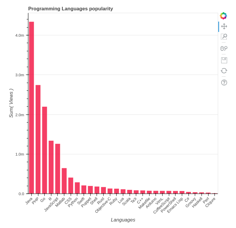
So, if we remove C from the consideration and look at other languages, we can see the following picture:
Evaluation. Java made it with over 4 million views daily, PHP and Go have over 2 million, R and JavaScript close up the “million scorers” list.
Daily Page Views vs Google Ranking
Let’s now take a look at the connection between the number of daily views and Google ranking of blogs. Logically, less popular blogs should be further in ranking, It’s not so easy though, as other factors influence ranking as well, for example, if the article in the less popular blog is more recent, it’ll likely pop up first.
The data preparation is performed in the following fashion:
def get_languages_popularity(data):
    query_sorted_data = sorted(data, key=itemgetter('query'))
    result = {'languages': [], 'views': []}
    popularity = []
    for k, group in groupby(query_sorted_data, key=itemgetter('query')):
        group = list(group)
        daily_page_views = map(lambda r: int(r['daily_page_views']), group)
        total_page_views = sum(daily_page_views)
        popularity.append((group[0]['query'], total_page_views))
    sorted_popularity = sorted(popularity, key=itemgetter(1), reverse=True)
    languages, views = zip(*sorted_popularity)
    result['languages'] = languages
    result['views'] = views
    return result
view rawanalysis.py hosted with
by GitHub
The function accepts scraped data and list of languages to consider. We sort the data in the same way we did for languages popularity. Afterwards, in a similar language grouping loop, we build (rank, views_number) tuples (with 1-based ranks) that are being converted to 2 separate lists. This pair of lists is then written to the resulting dictionary.
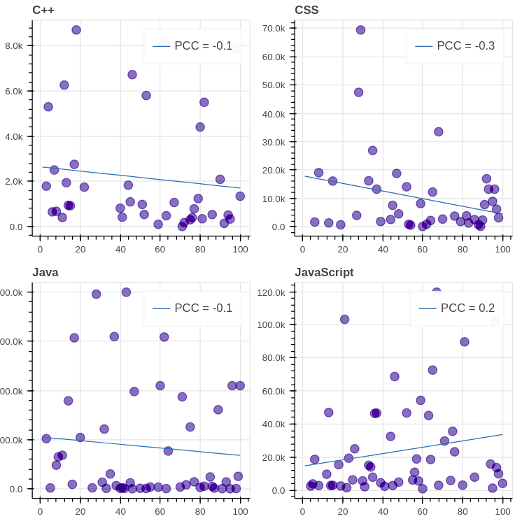
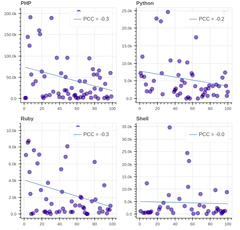
The results for the top 8 GitHub languages (except C) are the following:
Evaluation. We see that the PCC (Pearson correlation coefficient) of all graphs is far from 1/-1, which signifies lack of correlation between the daily views and the ranking. It’s important to note though that in most of the graphs (7 out of 8) the correlation is negative, which means that decrease in ranking leads to decrease in views indeed.
Conclusion
So, according to our analysis, Java is by far most popular programming language, followed by PHP, Go, R and JavaScript. Neither of top 8 languages has a strong correlation between daily views and ranking in Google, so you can definitely get high in search results even if you’re just starting your blogging path. What exactly is required for that top hit a topic for another discussion though.
These results are quite biased and can’t be taken into consideration without additional analysis. At first, it would be a good idea to collect more traffic feeds for an extended period of time and then analyze the mean (median?) values of daily views and rankings. Maybe I’ll return to it sometime in the future.
References
-
Scraping:
-
blog.scrapinghub.com: Handling Javascript In Scrapy With Splash
-
Traffic estimation:
-
quora.com: What are the best free tools that estimate visitor traffic…
via: https://www.databrawl.com/2017/10/08/blog-analysis/
作者:Serge Mosin 译者:译者ID 校对:校对者ID


